
SVM学习笔记
SVM(Support Vector Machine),即支持向量机,是在分类与回归分析中分析数据的监督式学习模型与相关的学习算法。SVM模型是一个非概率二元线性分类器,若从空间角度理解,SVM模型将样本表示为空间中的点,并试图找出一个最优的超平面来分隔样本,基于样本落在间隔的哪一侧,来预测所属的类别。
对于支持向量机来说,数据点若是$p$维向量,我们用$p−1$维的超平面来分开这些点。但是可能有许多超平面可以把数据分类。最佳超平面的一个合理选择就是以最大间隔把两个类分开的超平面。因此,SVM选择能够使离超平面最近的数据点的到超平面距离最大的超平面。
1)SVM模型
原理推导
由于SVM模型是一个非概率二元线性分类器,可以设有一个最优的参数组合$(w^,b^)$,使得分界最优,则该超平面$Η$可以用下式表示:
\[\{\vec{x}|\vec{w^*}^T\vec{x}+b^*=0\}\]易知$\vec{w^*}⊥H$。
如下图,对该Hyperplane,为使其分类效果达到最优,我们需要使其两侧的样本点到它的距离$margin$最大。
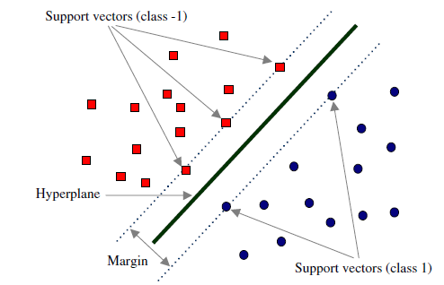
对于SVM模型来说,真正重要的是$Margin$内的样本点,即靠近超平面的点,这些样本点便是支持向量(Support Vector)。支持向量对模型起着决定性的作用,这也是“支持向量机”名称的由来。
为求支持向量到超平面的距离,过样本点作与超平面平行的平面,可以表示为:
\[\{\vec{w}^T\vec{x}+b=h(\vec{x})\}\]如图,假设$\vec{x}$在$H$的右侧,则有:
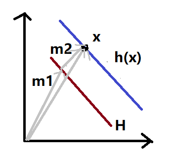
假设$\vec{x}$在$H$的左侧,则有:
\[r=-\frac{h(\vec{x})}{||\vec{w}||}=||\vec{m_2}||\]故写成:
\[d_{H-h(\vec{x})} = yr = \frac{y(\vec{w^T}\vec{x}+b)}{||\vec{w}||},y∈\{-1,1\}\]计算最大间隔及其对应的最优参数:
\[Margin = d_{{H-h(\vec{x})}_{min}}=min_l\frac{y^l(\vec{w^T}\vec{x}+b)}{||\vec{w}||}\] \[(\vec{w^*},\vec{b^*})=argmax_{\vec{w},b} \frac{1}{||\vec{w}||} min_l[{y^l(\vec{w^T}\vec{x}+b)}]\]该问题可以根据拉格朗日对偶性,转化为二次凸优化问题:
\[min_{\vec{w},b}\frac{1}{2}||\vec{w}||^2 s.t. y^l(\vec{w^T}\vec{x}+b)≥1,\forall l\]得到最优超平面对应的参数值$(w^,b^)$,最终的预测值为:
\[\hat{y(\vec{x})}=sign(\vec{w^*}^T\vec{x}+b^*)\]实践
在实践中,支持向量机学习方法有一些由简至繁的模型:
- 线性可分SVM
当训练数据线性可分时,通过硬间隔(hard margin)最大化可以学习得到一个线性分类器,即硬间隔SVM,即上述方法。
- 线性SVM
当训练数据不能线性可分但是可以近似线性可分时,通过软间隔(soft margin)最大化也可以学习到一个线性分类器,即软间隔SVM。
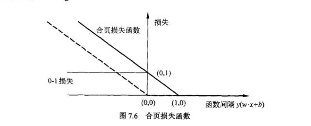
相比硬间隔,软间隔放宽了硬间隔最大化的条件,允许少量样本不满足约束$s.t. y^l(\vec{w^T}\vec{x}+b)≥1,\forall l$。为使这些样本点尽可能少,需要在优化目标函数中新增一个对这些点的惩罚项。常用的损失函数是hinge loss(合页损失),$Loss_{hinge}(z)=max(0,1-z)$。
要使软间隔最大化,优化目标将形如:
\[min_{W,b,\xi}\frac{1}{2}||W||^2+C\sum^n_{i=1}{\xi_i} s.t.y^i(\vec{X_i}^T\vec{W}+b)≥1-\xi_i,\forall i, \xi_i≥0\]- 非线性SVM
当训练数据线性不可分时,通过使用核技巧(kernel trick)和软间隔最大化,可以学习到一个非线性SVM。
通过核函数,支持向量机可以将特征向量映射到更高维的空间中,使得原本线性不可分的数据在映射之后的空间中变得线性可分。假设原始向量为x,映射之后的向量为z,这个映射为:
\[\boldsymbol{z} = \varphi(\boldsymbol{x})\]在实现时不需要直接对特征向量做这个映射,而是用核函数对两个特征向量的内积进行变换,这样做等价于先对向量进行映射然后再做内积:
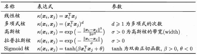
\[K(x_i,x_j)=K(x_i^Tx_j)=\phi(x_i)^T\phi(x_j)\]在这里K为kernel核函数。常用的非线性核函数有多项式核,高斯核(也叫径向基函数核,RBF)。下表列出了各种核函数的计算公式:
若想训练一个多分类模型,也可将多个SVM模型进行组合,得到多个划分超平面。
2)Hinge Loss
在机器学习中,hinge loss作为一个损失函数(loss function),通常被用于最大间隔算法(maximum-margin),而最大间隔算法又是SVM(支持向量机support vector machines)用到的重要算法。事实上,SVM的学习算法有两种解释,除了间隔最大化与拉格朗日对偶之外,便是Hinge Loss。
Hinge loss专用于二分类问题,标签值$y_i=±1$,预测值$\hat{y_i}=\boldsymbol{x_i}\boldsymbol{w}+b∈R$,$\boldsymbol{x_i}\in R^{1\times number\ of\ feature}$,$\boldsymbol{w}\in R^{number\ of\ feature\times 1}$对单个样本点,其损失函数为:
\[HingeLoss_\hat{y_i}=max(0,1-y_i\hat{y_i})\]从该式可以看出,该损失函数忽视正确分类且距离预测值分界点较远的样本点,只关注错误分类或正确分类但距离预测值分界点较近的样本点,这正是SVM中支持向量的概念。其体现了SVM中支持向量的稀疏性。
该函数在零点处不可导,但可以在编程时用梯度下降法实现。
在$1-y_i\hat{y_i}>0$时对其求导:
\[\frac{\partial L_i}{\partial \vec{w}}=-y_i\vec{x_i}^T\]使用梯度下降法优化参数,$\alpha$为学习率:
\[\boldsymbol{w_{i+1}}=\boldsymbol{w_i}-\alpha \sum_{i=l}^N\frac{\partial L_l}{\partial \boldsymbol{w_i}}\]若加上L2正则化项(软间隔),总损失函数为:
\[HingeLoss = \sum_{i=1}^N HingeLoss_{\hat{y_i}} + \lambda||\boldsymbol{w}||^2\]3)Cross-Entropy Loss
二分类
在二分类的情况下,模型最后需要预测的结果只有两种情况,对于每个类别我们的预测得到的概率为 p 和 1−p ,此时表达式为(log 的底数是 e):
\[L=\frac{1}{N}∑_iL_i=\frac{1}{N}\sum_i^N−[y_i⋅log(p_i)+(1−y_i)⋅log(1−p_i)]\]其中: -$ y_i$ —— 表示样本 $i$ 的$label$,正类为 $1$ ,负类为 $0$ - $p_i$ —— 表示样本 $i$ 预测为正类的概率
在交叉熵模型中,通过$z_i=\vec{x_i}\vec{w}+b$得到线性的预测值,再用$\sigma(z)$转换为概率值$p_i$,在二分类情况下,一般使用sigmoid函数:
\[p_i=\sigma(z_i)=sigmoid(z_i)=\frac{1}{1+e^{-z_i}}\] \[\frac{\partial p_i}{\partial z_i}=\sigma'(z_i) =\sigma(z_i)(1-\sigma(z_i))=p_i(1-p_i)\]对损失函数求导:
\[\frac{\partial L_i}{\partial \boldsymbol w}=\frac{\partial L_i}{\partial p_i}\frac{\partial p_i}{\partial z_i}\frac{\partial z_i}{\partial \boldsymbol w}\] \[\frac{\partial L_i}{\partial \boldsymbol w}=(-\frac{y_i}{p_i}+\frac{1-y_i}{1-p_i})p_i(1-p_i)\boldsymbol x_i^T\] \[\frac{\partial L_i}{\partial \boldsymbol w}=(p_i-y_i)\boldsymbol x_i^T\]使用梯度下降法优化参数,$\alpha$为学习率:
\(\boldsymbol{w_{i+1}}=\boldsymbol{w_i}-\alpha \sum_{l=1}^N\frac{\partial L_l}{\partial \boldsymbol{w_i}}\) 若加上L2正则化项(软间隔),总损失函数为:
{% raw %} \(CrossEntropy Loss = \frac{1}{N}∑_i^T−[y_i⋅log(p_i)+(1−y_i)⋅log(1−p_i)] + \lambda||\boldsymbol{w}||^2\)
多分类
多分类的情况实际上就是对二分类的扩展:
\[L=\frac{1}{N}∑_iL_i=-\frac{1}{N}∑_i∑_{c=1}^My_{ic}log(p_{ic})\]其中: - $M$ ——类别的数量 - $y_{ic}$ ——符号函数( 0 或 1 ),如果样本 $i$ 的真实类别等于 $c$ 取 $1$ ,否则取 $0$ - $p_{ic}$ ——观测样本 $i$ 属于类别 $c$ 的预测概率
4)库函数
1
2
3
from sklearn import svm

model=svm.SVC(*, C: *float* = 1, kernel: *str* = "rbf", degree: *int* = 3, gamma: *str* = "scale"...)
在SVC函数中,注意到几个参数:
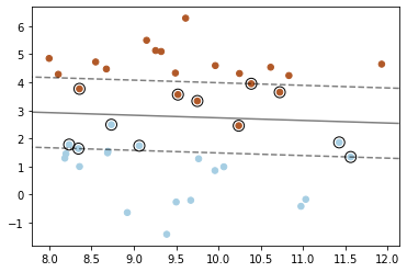
C:C是惩罚系数,即对误差的宽容度。c越高,说明越不能容忍出现误差,容易过拟合。C越小,容易欠拟合。C过大或过小,泛化能力变差。C的默认取值为1.0。
C=0.1 ![img]()
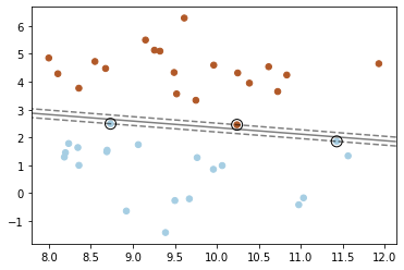
C=1000 ![img]()
kernel:linear(线性核)、poly(多项式核)、rbf(径向基核函数)、sigmoid(Sigmoid核)、precomputed(如果使用precomputed模式,也就是不传入函数,而直接传入计算后的核,那么参与这个核计算的数据集要包含训练集和测试集),默认为rbf(高斯核)。
degree:如果选择多项式核,则需要进一步设置多项式的次数这个参数——
degree,默认为3。gamma:gamma是选择RBF函数作为kernel(高斯核函数)后,该函数自带的一个参数。隐含地决定了数据映射到新的特征空间后的分布,gamma越大,支持向量越少,gamma值越小,支持向量越多。支持向量的个数影响训练与预测的速度。
5)手动实现
Hinge Loss线性分类模型
模型
预测值:$f(X;w,b)=sign(Xw+b)$
$w’=w⊕b$
$X’=X⊕[1,..,1]$
则模型可化为: $f(X’;w’)=sign(X’w’)$
算法流程
读取、分析、导入数据
随机初始化对应维度的权重$\vec{w}$与偏置$b$
用train set训练模型,利用梯度下降算法,以Hinge Loss为损失函数不断更新迭代$\vec{w}$参数
\[\frac{\partial L_i}{\partial \vec{w}}=-y_i\vec{x_i}^T,1-y_i\hat{y_i}>0\] \[\boldsymbol{w_{i+1}}=\boldsymbol{w_i}-\alpha \sum_{i=l}^N\frac{\partial L_l}{\partial \boldsymbol{w_i}}\]直到Loss值收敛,得到构造最优分类超平面的最优的权重$\vec{w}$
记录每次迭代的平均损失值,绘制Loss值趋势图
用test set验证模型的准确性
代码
实现一个Hinge Loss线性分类器。
1
2
3
4
5
6
7
8
9
10
11
12
13
14
15
16
17
18
19
20
21
22
23
24
25
26
27
28
29
30
31
32
33
34
35
36
37
38
39
40
41
42
43
44
45
46
47
48
49
50
51
52
class LinearClassifier():
    def __init__(self, feat):
        self.w = np.random.rand(feat+1,1)  # initialize the weight; shape like (feat,1)
        self.feat = feat
    def train(self, X_, y, alpha=1e-5, max_iter=100, reg=False, lamb=0.5):
        """train the model

        Args:
            X (numpy.ndarray): input of trainset, shape like (sample,feat).
            y (numpy.ndarray): label of trainset, shape like (sample,1).
            alpha (float,optional): learning rate. Defaults to 1e-3.
            max_iter (int, optional): epoch. Defaults to 100.
            reg (bool,optional): whether to L2-regularize. Defaults to True.
            lamb (float, optional): parameter of L2-regularization. Defaults to 0.5.
        """

        X = np.column_stack((X_,np.ones((X_.shape[0],1))))
        sample = X.shape[0]
        for epoch in range(max_iter):
            avg = 0
            # Gradient Descend
            for i in range(sample):
                x = X[i].reshape(1,self.feat+1)
                loss = max(0,1 - (y[i] * np.dot(x,self.w)[0][0]))
                if loss != 0:
                    self.w -= alpha * (-y[i]*x.T)
                if reg:
                    self.w *= 1-alpha*lamb*2
                    loss += lamb*np.linalg.norm(self.w,2)
                avg+=loss
            los.append(avg/sample)

    def predict(self,X_):
        """predict label of X_ by trained weights

        Args:
            X_ (np.ndarray): input of dataset, shape like (sample,feat).

        Returns:
            np.ndarray: predicted label of X_, shape like(sample,1).
        """

        X = np.column_stack((X_,np.ones((X_.shape[0],1))))
        Y = np.dot(X,self.w)
        Y[Y>0] = 1
        Y[Y<=0] = -1
        return Y

    def Ascore(self, y, pre): # Accuracy 准确率:分类器正确分类的样本数与总样本数之比
        sample = y.shape[0]
        error = np.linalg.norm(y-pre.ravel(),1)/2
        return 1-error/sample
Cross-Entropy Loss线性分类模型
模型
预测值:$f(X;w,b)=sign(sigmoid(Xw+b)-0.5)$
$w’=w⊕b$
$X’=X⊕[1,..,1]$
则模型可化为: $f(X’;w’)=sign(sigmoid(X’w’+b)-0.5)$
算法流程
读取、分析、导入数据
随机初始化对应维度的权重$\vec{w}$与偏置$b$
用train set训练模型,利用梯度下降算法,以为Cross-Entropy Loss损失函数不断更新迭代$\vec{w}$参数
\[\frac{\partial L_i}{\partial \boldsymbol w}=(p_i-y_i)\boldsymbol x_i^T\] \[\boldsymbol{w_{i+1}}=\boldsymbol{w_i}-\alpha \sum_{i=l}^N\frac{\partial L_l}{\partial \boldsymbol{w_i}}\]直到Loss值收敛,得到构造最优分类超平面的最优的权重$\vec{w}$
记录每次迭代的平均损失值,绘制Loss值趋势图
用test set验证模型的准确性
代码
实现一个Cross-Entropy Loss线性分类器。
1
2
3
4
5
6
7
8
9
10
11
12
13
14
15
16
17
18
19
20
21
22
23
24
25
26
27
28
29
30
31
32
33
34
35
36
37
38
39
40
41
42
43
44
45
46
47
48
49
50
51
52
53
54
55
56
57
class LinearClassifier():
    def __init__(self, feat):
        self.w = np.random.rand(feat+1,1)  # initialize the weight; shape like (feat,1)
        self.feat = feat

    def sigmoid(self,z):
        warnings.filterwarnings('ignore')
        return 1 / (1 + np.exp(-z))

    def train(self, X_, y, alpha=1e-5, max_iter=100, reg=False, lamb=0.2):
        """train the model

        Args:
            X (numpy.ndarray): input of trainset, shape like (sample,feat).
            y (numpy.ndarray): label of trainset, shape like (sample,1).
            alpha (float,optional): learning rate. Defaults to 1e-3.
            max_iter (int, optional): epoch. Defaults to 100.
            reg (bool,optional): whether to L2-regularize. Defaults to True.
            lamb (float, optional): parameter of L2-regularization. Defaults to 0.5.
        """

        X = np.column_stack((X_,np.ones((X_.shape[0],1))))
        sample = X.shape[0]
        for epoch in range(max_iter):
            avg = 0
            # gradient descend
            for i in range(sample):
                x = X[i].reshape(1,self.feat+1)
                z = np.dot(x,self.w)[0][0]
                p = self.sigmoid(z)+1e-8 #防止p=0造成loss中log函数错误
                loss = -y[i]*log(p)-(1-y[i])*log(1-p)
                self.w -= alpha * (p-y[i])*x.T
                if reg:
                    self.w *= 1-alpha*lamb*2
                    loss += lamb*np.linalg.norm(self.w,2)
                avg+=loss
            los.append(avg/sample)

    def predict(self,X_):
        """predict label of X_ by trained weights

        Args:
            X_ (np.ndarray): input of dataset, shape like (sample,feat).

        Returns:
            np.ndarray: predicted label of X_, shape like(sample,1).
        """
        X = np.column_stack((X_,np.ones((X_.shape[0],1))))
        Y = self.sigmoid(np.dot(X,self.w))
        Y[Y>0.5] = 1
        Y[Y<=0.5] = 0
        return Y

    def Ascore(self, y, pre): #Accuracy 准确率:分类器正确分类的样本数与总样本数之比
        sample = y.shape[0]
        error = np.linalg.norm(y-pre.ravel(),1)
        return 1-error/sample